Phrase-based Model: Difference between revisions
No edit summary |
No edit summary |
||
| (22 intermediate revisions by 2 users not shown) | |||
| Line 1: | Line 1: | ||
{{Infobox | {{Infobox | ||
|title = Lecture | |title = Lecture 9: Phrase-based model | ||
|image = [[File:computer-copies.png|200px]] | |image = [[File:computer-copies.png|200px]] | ||
|label1 = Lecture video: | |label1 = Lecture video: | ||
| Line 12: | Line 12: | ||
== Phrase Extraction == | == Phrase Extraction == | ||
PBMT uses '''phrases''' as the basic unit of translation. Phrases are simply sequences of words which have been observed in the training data, they don't correspond to any linguistic notion of phrases. | PBMT uses '''phrases''' as the basic unit of translation. Phrases are simply contiguous sequences of words which have been observed in the training data, they don't correspond to any linguistic notion of phrases. | ||
In order to obtain a '''phrase table''' (a probabilistic dictionary of phrases), we need [[Word Alignment|word-aligned]] parallel data. | In order to obtain a '''phrase table''' (a probabilistic dictionary of phrases), we need [[Word Alignment|word-aligned]] parallel data. Using the alignment links, a simple heuristic is applied to extract '''consistent''' phrase pairs. Consider the word-aligned example sentence: | ||
[[File:phrase-extraction.png|400px]] | |||
Phrase pairs are contiguous spans where all alignment points from the source side of the span fall within its target side and vice versa. These are examples of phrases consistent with this word alignment: | |||
[[File:phrase-extraction-okay.png|400px]] [[File:phrase-extraction-okay2.png|400px]] | |||
On the other hand, if either a source word or a target word is aligned outside of the current span, the phrase cannot be extracted. The conflicting alignment points are drawn in yellow: | |||
[[File:phrase-extraction-short.png|400px]] [[File:phrase-extraction-long.png|400px]] | |||
In practice, only phrases up to a certain length are extracted (e.g. 7 words). Longer phrases would hardly ever be used by the translation model (unless it was presented with a sentence from the training data) and the phrase table would be extremely large. | |||
== Phrase Scoring == | |||
Once we have extracted all consistent phrase pairs from our training data, we can assign translation probabilities to them using maximum likelihood estimation. To estimate the probability of phrase <math>e</math> being the translation of phrase <math>f</math>, we simply count: | |||
<math> | |||
P(e|f) = \frac{\text{count}(e,f)}{\text{count}(f)} | |||
</math> | |||
The formula tells us to simply count how many times we saw <math>f</math> translated as <math>e</math> in our training data and divide that by the number of times we saw <math>f</math> in total. | |||
In practice, several other scores are also computed (including the reverse phrase translation probability <math>P(f|e)</math>) but that's a topic for another lecture. | |||
== Decoding == | |||
When we get an input sentence for translation, the first step is to look up '''translation options''' (possible translations) for each source span in the phrase table. These can be thought of as jigsaw puzzle pieces which are combined to get as good final translation as possible. The task for the '''decoder''' (the translation program) is to find a combination which covers the whole input sentence and is the most probable according to the model (this procedure is usually called decoding). | |||
Here we describe the stack-based '''beam search''' algorithm which is commonly used for phrase-based decoding, although other algorithms exist. | |||
=== Overview === | |||
The search begins with an empty hypothesis: no part of the input is covered and nothing has been produced. We can start covering the input sentence by translating any span, and for each span, we can choose any of its possible translations. The decoder produces all of these partial hypotheses. | |||
In the next step, we try to expand our partial translations further by covering the remaining parts of the input sentence. We continue expanding our partial hypotheses until we cover the whole source sentence. We choose the most probable translation. | |||
In the following example, we try to translate the Czech sentence: | |||
: ''Honza miluje Marii'' | |||
With the following phrase table: | |||
Honza ||| John | |||
Honza ||| Johny | |||
miluje ||| loves | |||
miluje ||| is fond of | |||
miluje ||| likes | |||
Marii ||| Mary | |||
This is an excerpt of the space where the decoder searches for the best translation. One (the most reasonable) full translation is illustrated but the decoder theoretically needs to evaluate all possible combinations. | |||
[[File:beam-search.png|350px]] | |||
Note that we keep track of covered input spans in a Boolean array (1 for covered words, 0 for untranslated ones) -- we know that we have a full translation once the '''coverage vector''' has no more zeroes. | |||
=== Stacks, Pruning === | |||
It is obvious that with realistic sentence lengths and translation dictionaries, the search space very quickly explodes and it becomes impossible to go through all the possible combinations of span translations and their orderings. | |||
First, we need to impose a limit on reordering (how far we can jump in the input), otherwise the search would be hopelessly intractable. In practice, the limit is set to roughly 6 words. | |||
Furthermore, we need to prune our partial hypotheses as there are still too many combinations. Our model assigns a score to each of them (more on that in later lectures) so we can sort our translations according to it and only keep several most promising candidates. | |||
However, it would be unfair to compare a score of a full translation with a partial hypothesis that e.g. only had to translate one phrase. The full hypothesis contains more decisions => more uncertainty => almost surely, the full translation has a lower score. For this reason, partial hypotheses are organized into '''stacks''' according to the number of covered input words. For each number, we have a separate stack. That way, only hypotheses which cover the same "amount" of input are compared. | |||
The algorithm can then proceed from stack "0" (which contains the empty hypothesis) to the final stack where full hypotheses compete for the best score. Each stack has a limited size which keeps the search tractable. | |||
There is one more caveat -- not all input words (or spans -- phrases) are created equal. Some are difficult to translate and some only have one or a few possible translations. To account for this discrepancy, phrase-based decoders estimate the '''future cost''' of translating the remainder of the input sentence. This estimation is based on the score of the most probable translation of the remaining spans and can be efficiently pre-computed using dynamic programming. Without accounting for future cost, hypotheses which translate the easiest words first would dominate the stacks and the search would lead to heavily suboptimal solutions. | |||
=== A Real Example === | |||
The following search graphs were exported from Moses when translating the sentence: | |||
: ''Ze schůze sněmovny vypadl horní zákon.'' (The mining law was dropped from the meeting of the House.) | |||
The graphs differ in stack limits (1, 30, 50) -- the maximum number of partial hypotheses on each stack. For clarity, we show the union of all translations considered by any of the systems in dotted lines. Full lines represent the translations considered by that particular system. | |||
For example, the first system (stack limit 1) proposes just a single translation: | |||
: ''the meeting of the House of the upper law . fell'' | |||
[[File:merged-0001.png|800px]] | |||
This is not a good translation and systems with higher stack limits do not even consider it. Because they can keep more than one-best candidate on each stack, they are able to find better-scoring combinations of translation options and this partial translation is pruned away before covering the whole input sentence. See the search graphs for stack limit 30 and 50 for comparison: | |||
[[File:merged-0030.png|800px]] [[File:merged-0050.png|800px]] | |||
== See Also == | == See Also == | ||
* [http://www.statmt.org/book/slides/05-phrase-based-models.pdf Philipp Koehn's slides on PBMT] | * [http://www.statmt.org/book/slides/05-phrase-based-models.pdf Philipp Koehn's slides on PBMT] | ||
* [http://www.statmt.org/book/slides/06-decoding.pdf Decoding in PBMT] | |||
Latest revision as of 13:29, 29 April 2015
 | |
| Lecture video: |
web TODO Youtube |
|---|---|
Phrase-based machine translation (PBMT) is probably the most widely used approach to MT today. It is relatively simple and easy to adapt to new languages.
Phrase Extraction
PBMT uses phrases as the basic unit of translation. Phrases are simply contiguous sequences of words which have been observed in the training data, they don't correspond to any linguistic notion of phrases.
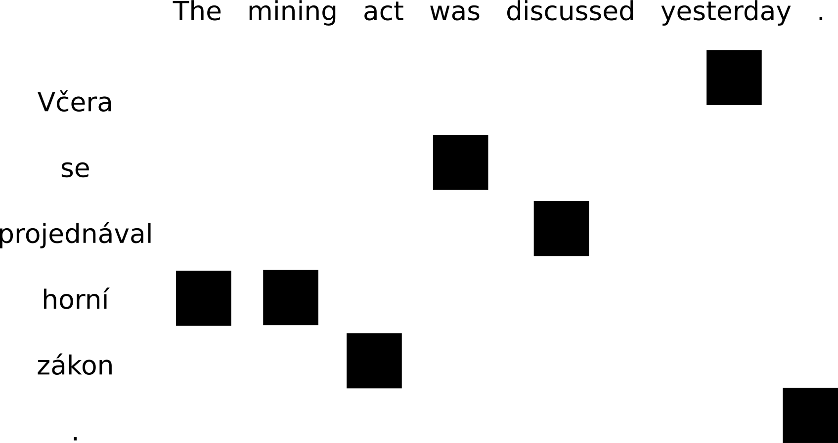
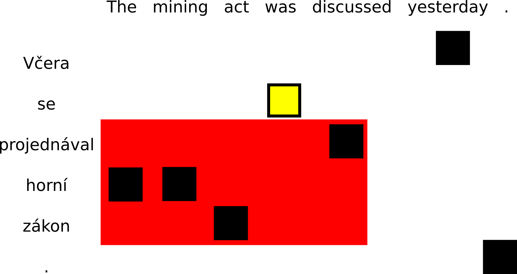
In order to obtain a phrase table (a probabilistic dictionary of phrases), we need word-aligned parallel data. Using the alignment links, a simple heuristic is applied to extract consistent phrase pairs. Consider the word-aligned example sentence:
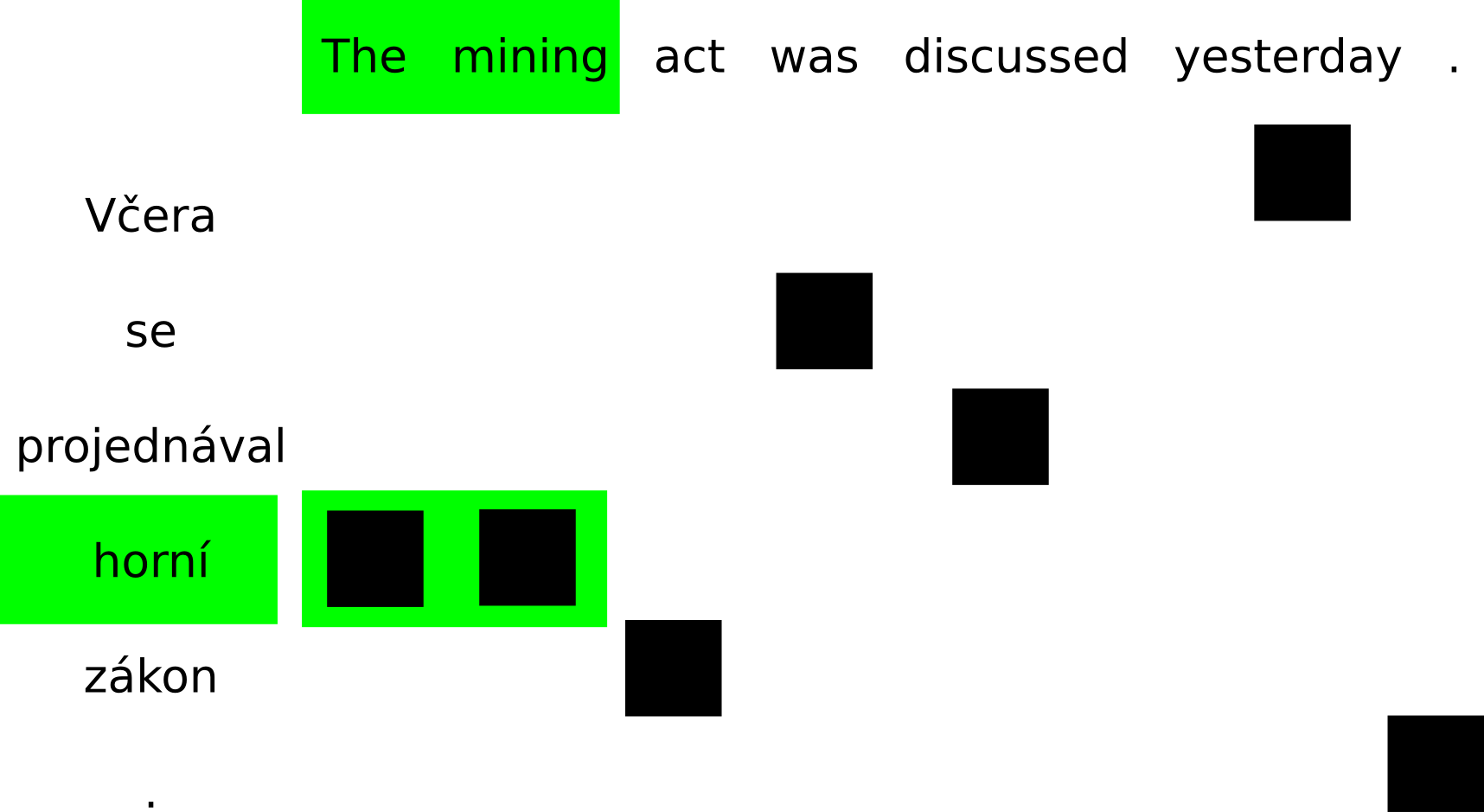
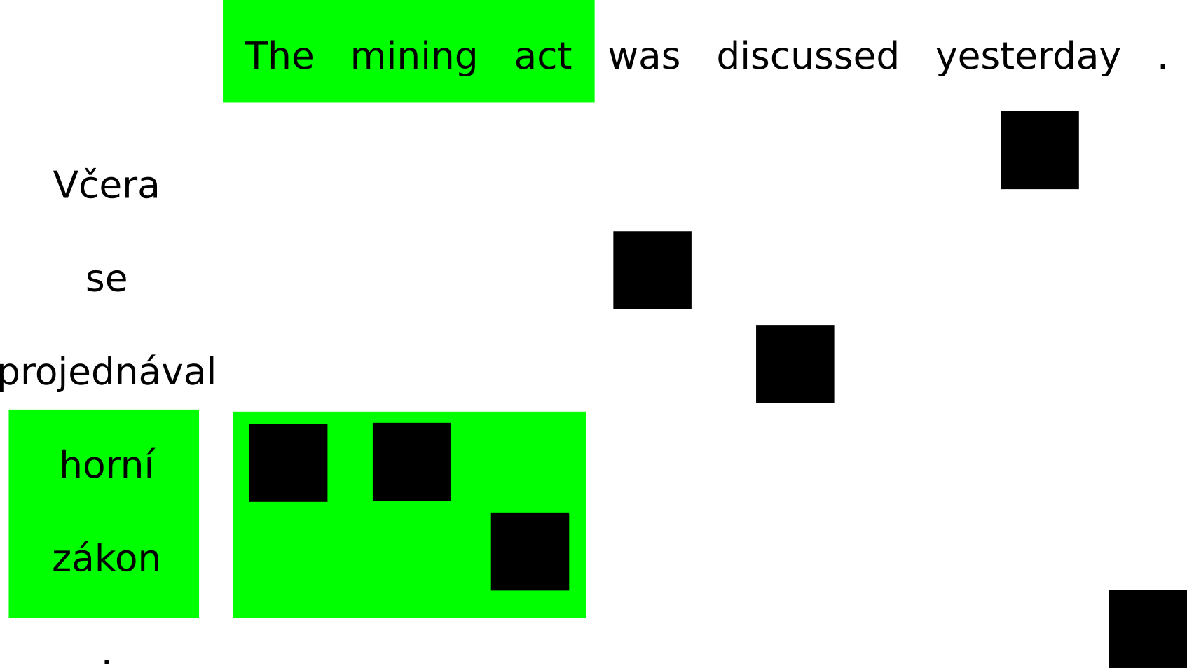
Phrase pairs are contiguous spans where all alignment points from the source side of the span fall within its target side and vice versa. These are examples of phrases consistent with this word alignment:
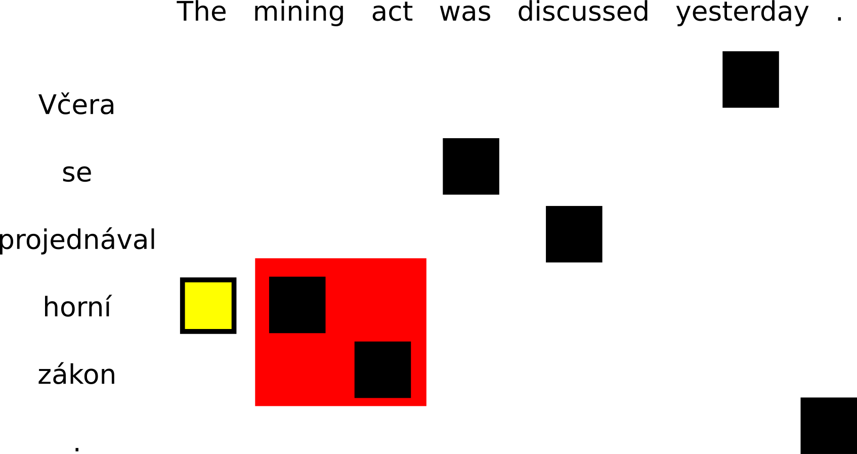
On the other hand, if either a source word or a target word is aligned outside of the current span, the phrase cannot be extracted. The conflicting alignment points are drawn in yellow:
In practice, only phrases up to a certain length are extracted (e.g. 7 words). Longer phrases would hardly ever be used by the translation model (unless it was presented with a sentence from the training data) and the phrase table would be extremely large.
Phrase Scoring
Once we have extracted all consistent phrase pairs from our training data, we can assign translation probabilities to them using maximum likelihood estimation. To estimate the probability of phrase being the translation of phrase , we simply count:
The formula tells us to simply count how many times we saw translated as in our training data and divide that by the number of times we saw in total.
In practice, several other scores are also computed (including the reverse phrase translation probability ) but that's a topic for another lecture.
Decoding
When we get an input sentence for translation, the first step is to look up translation options (possible translations) for each source span in the phrase table. These can be thought of as jigsaw puzzle pieces which are combined to get as good final translation as possible. The task for the decoder (the translation program) is to find a combination which covers the whole input sentence and is the most probable according to the model (this procedure is usually called decoding).
Here we describe the stack-based beam search algorithm which is commonly used for phrase-based decoding, although other algorithms exist.
Overview
The search begins with an empty hypothesis: no part of the input is covered and nothing has been produced. We can start covering the input sentence by translating any span, and for each span, we can choose any of its possible translations. The decoder produces all of these partial hypotheses.
In the next step, we try to expand our partial translations further by covering the remaining parts of the input sentence. We continue expanding our partial hypotheses until we cover the whole source sentence. We choose the most probable translation.
In the following example, we try to translate the Czech sentence:
- Honza miluje Marii
With the following phrase table:
 Honza ||| John
 Honza ||| Johny
 miluje ||| loves
 miluje ||| is fond of
 miluje ||| likes
 Marii ||| Mary
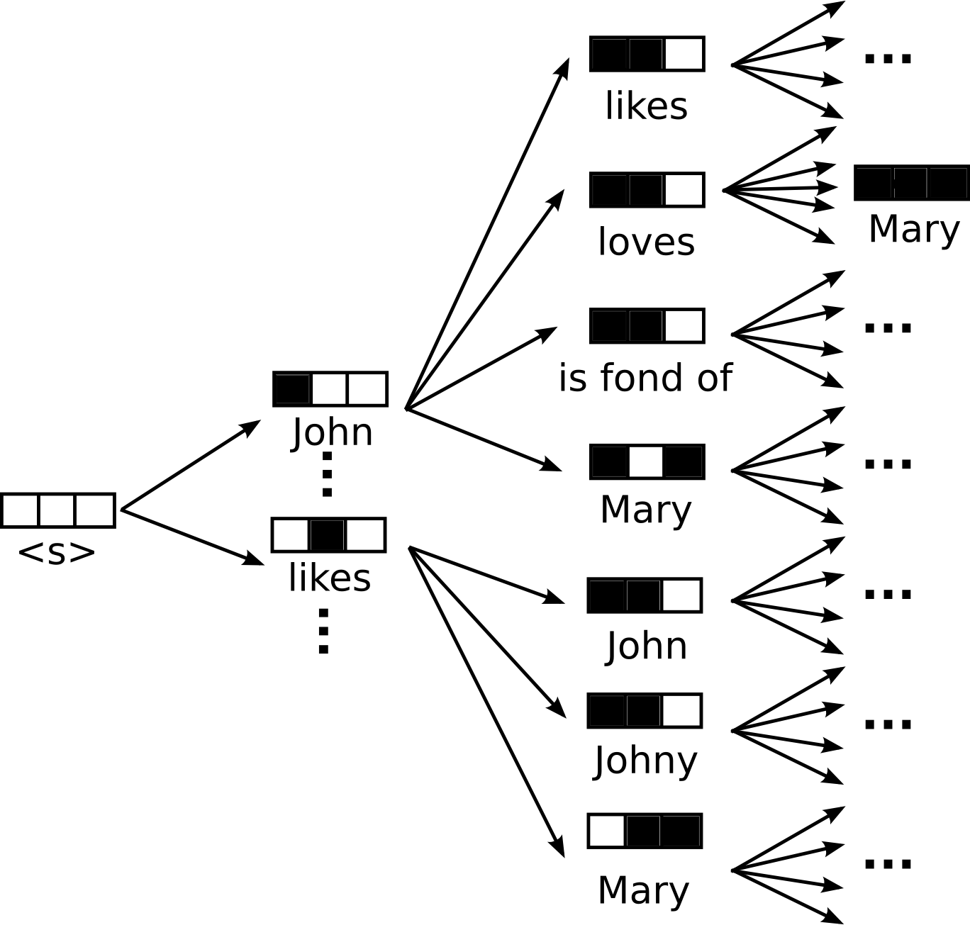
This is an excerpt of the space where the decoder searches for the best translation. One (the most reasonable) full translation is illustrated but the decoder theoretically needs to evaluate all possible combinations.
Note that we keep track of covered input spans in a Boolean array (1 for covered words, 0 for untranslated ones) -- we know that we have a full translation once the coverage vector has no more zeroes.
Stacks, Pruning
It is obvious that with realistic sentence lengths and translation dictionaries, the search space very quickly explodes and it becomes impossible to go through all the possible combinations of span translations and their orderings.
First, we need to impose a limit on reordering (how far we can jump in the input), otherwise the search would be hopelessly intractable. In practice, the limit is set to roughly 6 words.
Furthermore, we need to prune our partial hypotheses as there are still too many combinations. Our model assigns a score to each of them (more on that in later lectures) so we can sort our translations according to it and only keep several most promising candidates.
However, it would be unfair to compare a score of a full translation with a partial hypothesis that e.g. only had to translate one phrase. The full hypothesis contains more decisions => more uncertainty => almost surely, the full translation has a lower score. For this reason, partial hypotheses are organized into stacks according to the number of covered input words. For each number, we have a separate stack. That way, only hypotheses which cover the same "amount" of input are compared.
The algorithm can then proceed from stack "0" (which contains the empty hypothesis) to the final stack where full hypotheses compete for the best score. Each stack has a limited size which keeps the search tractable.
There is one more caveat -- not all input words (or spans -- phrases) are created equal. Some are difficult to translate and some only have one or a few possible translations. To account for this discrepancy, phrase-based decoders estimate the future cost of translating the remainder of the input sentence. This estimation is based on the score of the most probable translation of the remaining spans and can be efficiently pre-computed using dynamic programming. Without accounting for future cost, hypotheses which translate the easiest words first would dominate the stacks and the search would lead to heavily suboptimal solutions.
A Real Example
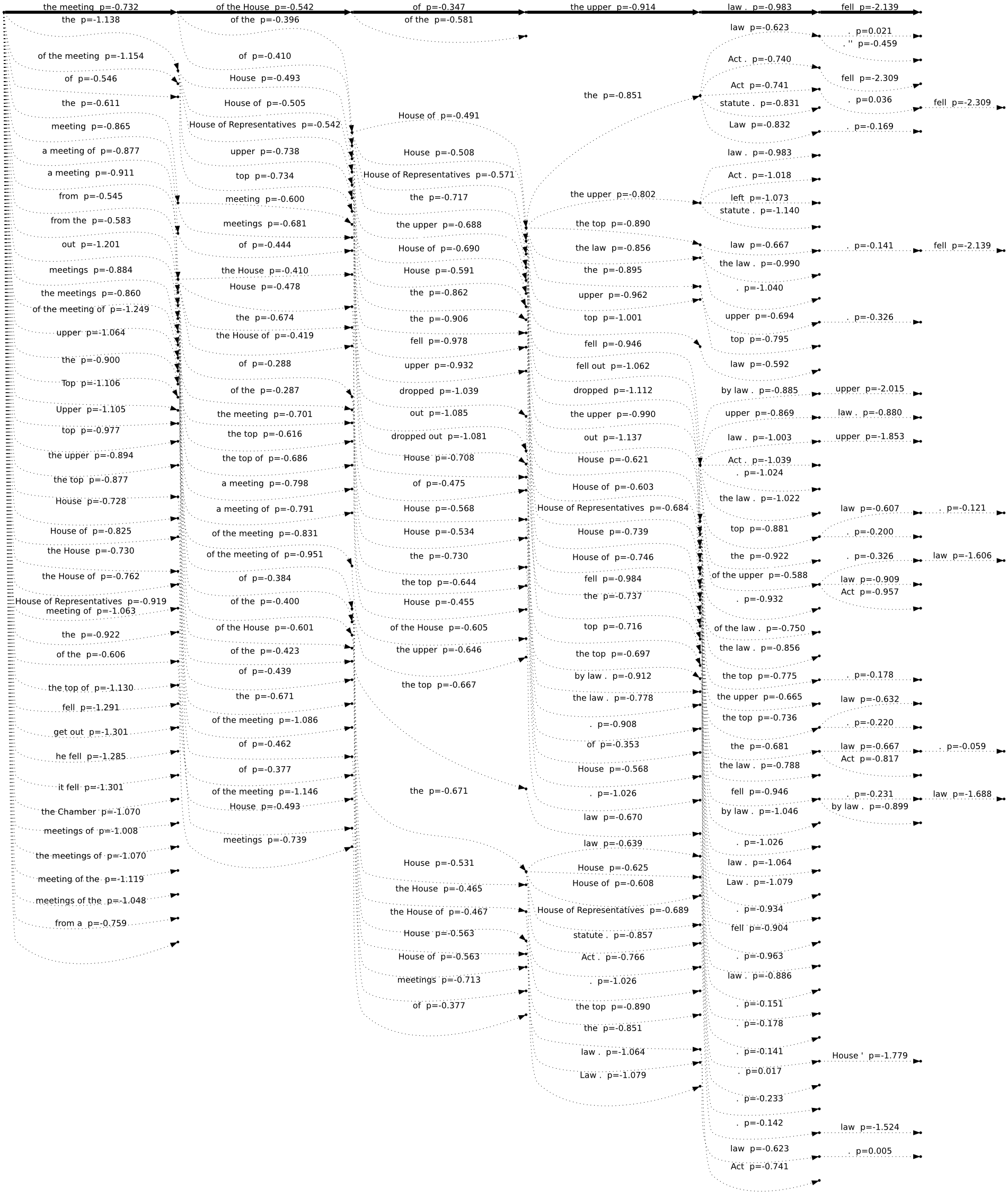
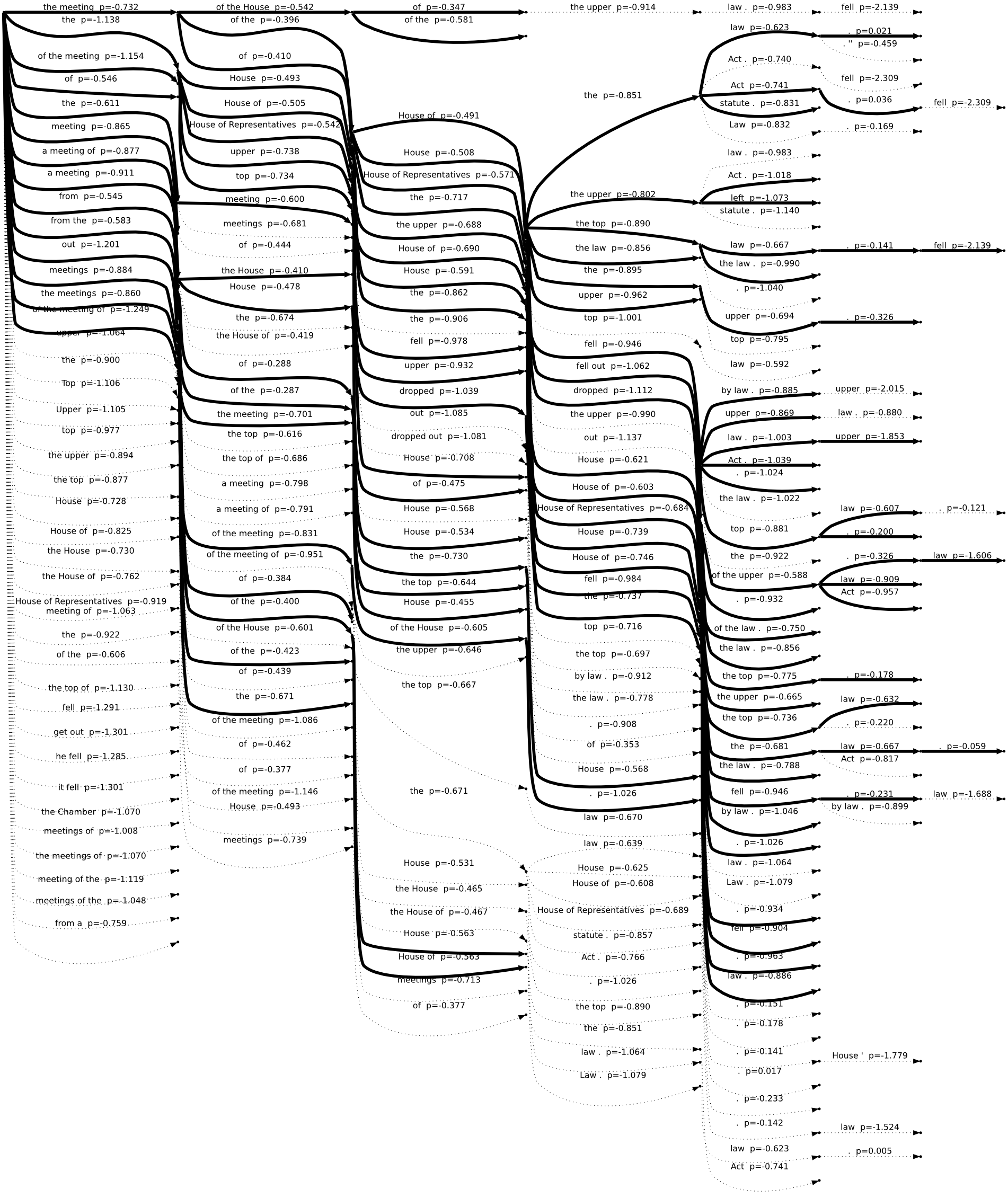
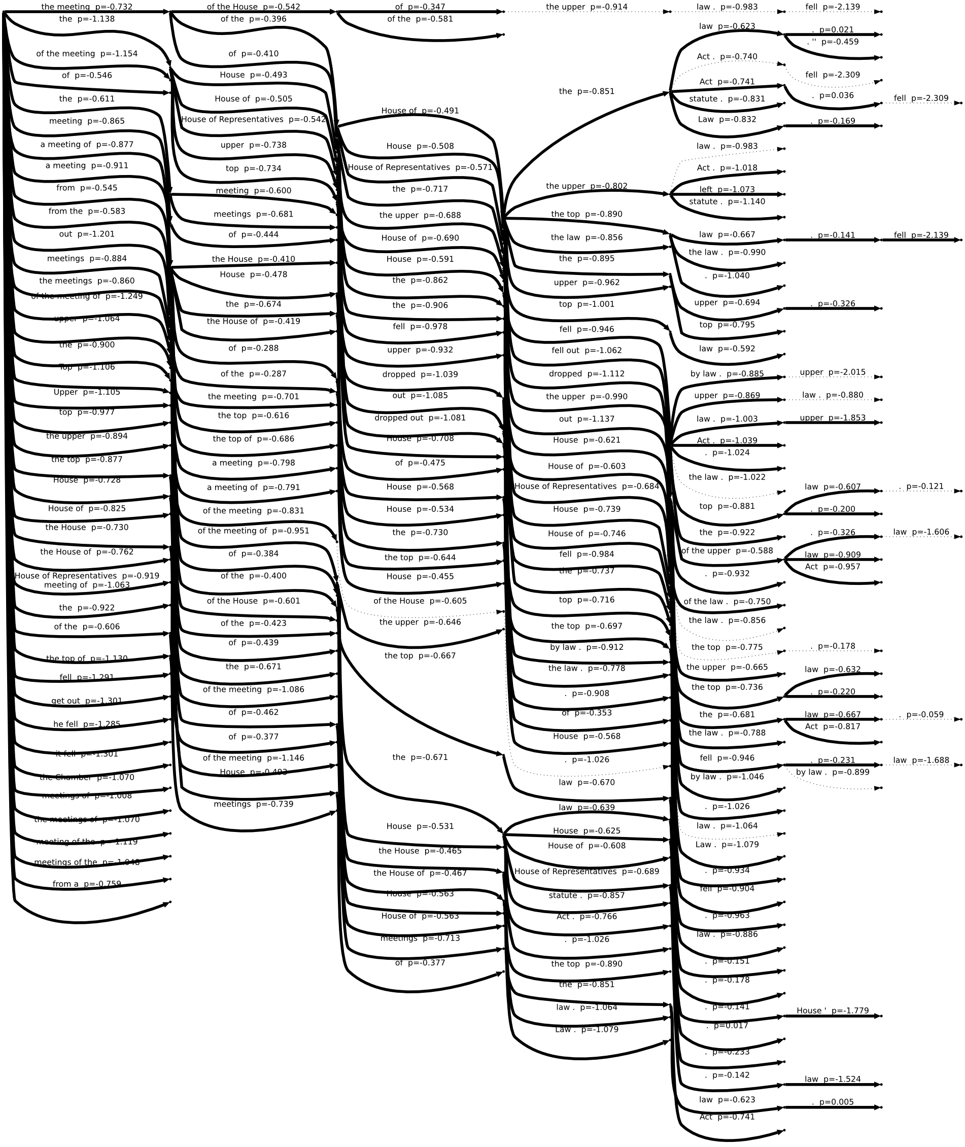
The following search graphs were exported from Moses when translating the sentence:
- Ze schůze sněmovny vypadl horní zákon. (The mining law was dropped from the meeting of the House.)
The graphs differ in stack limits (1, 30, 50) -- the maximum number of partial hypotheses on each stack. For clarity, we show the union of all translations considered by any of the systems in dotted lines. Full lines represent the translations considered by that particular system.
For example, the first system (stack limit 1) proposes just a single translation:
- the meeting of the House of the upper law . fell
This is not a good translation and systems with higher stack limits do not even consider it. Because they can keep more than one-best candidate on each stack, they are able to find better-scoring combinations of translation options and this partial translation is pruned away before covering the whole input sentence. See the search graphs for stack limit 30 and 50 for comparison:
